Debugging mode

Some configurations can be turned on to debug the simulator. As a result, you can get more console output from the simulation and visualizations such as coordinates and physics to help develop features or fix bugs. To receive debug messages, set debug=True in the config when creating the environment. In debug mode, the log_level will be changed to logging.DEBUG, so you will get more information from MetaDrive, Panda3D, and RenderPipeline in the console.

Debug physics

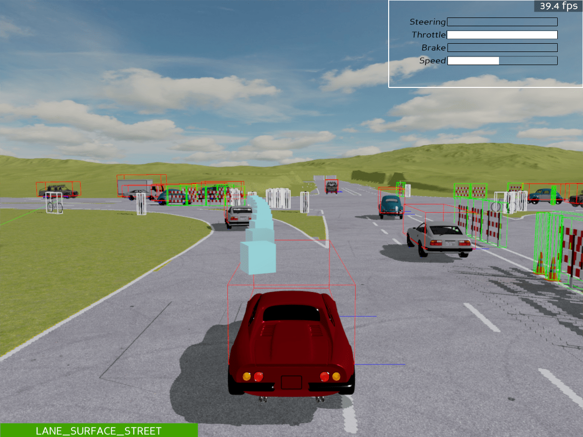
It is important to make sure that physics world is accurate. For example, objects should have accurate bounding boxes in order to ensure the collision detection is correct. Specifying debug=True in environment config can turn on the debug mode. In this mode, you can visualize the physics world by pressing 1 (the one near ~) on your keyboard. In the following example, we have automatically turned on the physics world visualizer for you by env.engine.toggleDebug(). Pressing 1 can turn if off.

from metadrive.envs.scenario_env import ScenarioEnv
import numpy as np
import os
render = not os.getenv('TEST_DOC')

# create real-world environment with debug mode turned on
env = ScenarioEnv(dict(use_render=render, debug=True)) 
env.reset(seed=0)
# turn on physics world visualizer
env.engine.toggleDebug()

try:
    for i in range(200):
        o,r,d,t,i = env.step([0,1])
        if d:
            break
finally:
    env.close()

The default debug mode only visualizes the object in the world called “dynamics physics world”. In this world, objects can have interactions following the physics law like collision, friction, and gravity. At the same time, there exists another physics world called “static physics world”, where objects won’t participate in collision and enjoy zero gravity. However, one can still query this world to know if an object in dynamics physics world has contact with objects in the static physics world. Therefore, we usually put objects that are still like crosswalks, lane lines and lanes in this world. As a result, we can know which lane the car is on or if it is on a lane line or sidewalk, while keep the simulation at a high FPS as we only step the dynamics physics world.

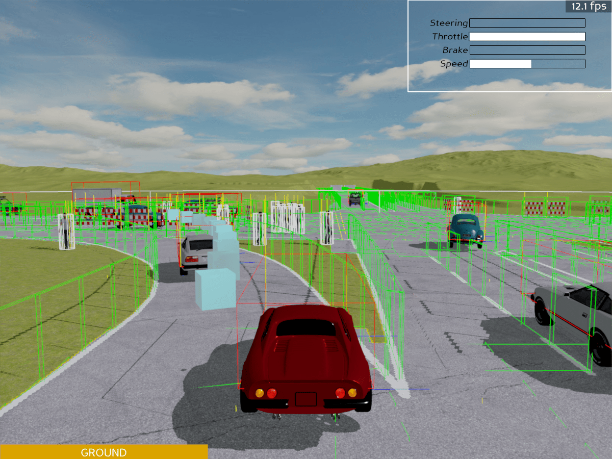
To visualize the dynamics physics world and static physics world together, we can turn on the config['debug_static_world']=True. The following example visualizes both physics worlds by adding objects which are supposed to be in static physics world to the dynamics physics world. You will also experience a FPS drop, which explains why we separate the physics world into two.

from metadrive.envs.scenario_env import ScenarioEnv
import numpy as np
import os
render = not os.getenv('TEST_DOC')

# create real-world environment with debug mode turned on
env = ScenarioEnv(dict(use_render=render, debug=True, debug_static_world=True)) 
env.reset(seed=0)
# turn on physics world visualizer
env.engine.toggleDebug()

try:
    for i in range(200):
        o,r,d,t,i = env.step([0,1])
        if d:
            break
finally:
    env.close()

There is a more aggressive option debug_physics_world to debug the physics engine. It will turn off all graphics and only keep the line frames representing physics bodies. Turn it on via debug_physics_world=True.

from metadrive.envs.scenario_env import ScenarioEnv
import numpy as np
import os
render = not os.getenv('TEST_DOC')

# create real-world environment with debug mode turned on
env = ScenarioEnv(dict(use_render=render, 
                       debug=True, 
                       debug_physics_world=True, 
                       debug_static_world=True)) 
env.reset(seed=0)
# turn on physics world visualizer
env.engine.toggleDebug()

try:
    for i in range(200):
        o,r,d,t,i = env.step([0,1])
        if d:
            break
finally:
    env.close()

Debug Panda3D

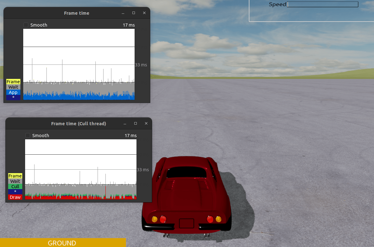
In addition to the errors raised from MetaDrive, sometimes the game engine, Panda3D, will throw errors and warnings about the rendering service. To enable the logging of Panda3D, set env_config["debug_panda3d"]=True. Besides, you can turn on Panda3D’s profiler via env_config["pstats"]=True and launch the pstats in the terminal. It can be used to analyze your program in terms of the time consumed for different functions like rendering, physics and so on, which is very useful if you are developing some graphics related features.

# launch pstats (bash)
!pstats

from metadrive.envs.base_env import BaseEnv
import os
render = not os.getenv('TEST_DOC')

# create environment
env = BaseEnv(dict(use_render=render, debug=True, debug_panda3d=True, pstats=True))

# reset environment
env.reset()
try:
    for i in range(1000):
        env.step(env.action_space.sample())
finally:
    env.close()

Show coordinates

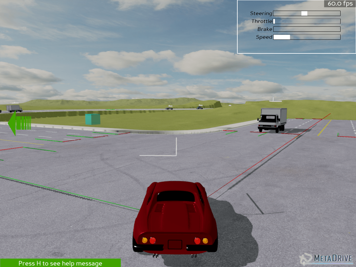
Coordinates are important for developing robotics systems. To show the coordinates for the map, the world and objects, please set show_coordinate=True when creating the environment. There are three types of coordinates will be shown:

World/global coordinates which moves with the car. The +x direction is marked in red and is longer. The +y direction is in green and shorter.
Lane coordinates marking the longitudinal and lateral direction of each lane. For each lane, the green line is the +longitudinal direction and the red line is +lateral direction.
Object’s local coordinate. The longer line points to +x direction and the shorter line points to +y direction.

from metadrive.envs.metadrive_env import MetaDriveEnv
from metadrive.policy.idm_policy import IDMPolicy
import os
test = os.getenv('TEST_DOC')


# create environment
env = MetaDriveEnv(dict(use_render=not test, 
                        show_coordinates=True, 
                        agent_policy=IDMPolicy,
                        num_scenarios=1,
                        map="XCO"))

# reset environment
env.reset()
try:
    for i in range(1000):
        o,r,d,t,_ = env.step([0,0])
        if d:
            break
finally:
    env.close()